Estoy tratando de implementar la eliminación de sombras en Python OpenCV usando el método de minimización de entropía de Finlayson, et. Alabama.:

"Imágenes intrínsecas por minimización de entropía", Finlayson, et. Alabama.

Parece que no puedo igualar los resultados del artículo. Mi gráfico de entropía no coincide con los del documento y obtengo la entropía mínima incorrecta.

¿Alguna idea? (Tengo mucho más código fuente y documentos a pedido)

#############
# LIBRARIES
#############
import numpy as np
import cv2
import os
import sys
import matplotlib.image as mpimg
import matplotlib.pyplot as plt
from PIL import Image
import scipy
from scipy.optimize import leastsq
from scipy.stats.mstats import gmean
from scipy.signal import argrelextrema
from scipy.stats import entropy
from scipy.signal import savgol_filter

root = r'\path\to\my_folder'
fl = r'my_file.jpg'

#############
# PROGRAM
#############
if __name__ == '__main__':

    #-----------------------------------
    ## 1. Create Chromaticity Vectors ##
    #-----------------------------------

    # Get Image
    img = cv2.imread(os.path.join(root, fl))
    img = cv2.cvtColor(img, cv2.COLOR_BGR2RGB)
    h, w = img.shape[:2]

    plt.imshow(img)
    plt.title('Original')
    plt.show()

    img = cv2.GaussianBlur(img, (5,5), 0)

    # Separate Channels
    r, g, b = cv2.split(img) 

    im_sum = np.sum(img, axis=2)
    im_mean = gmean(img, axis=2)

    # Create "normalized", mean, and rg chromaticity vectors
    #  We use mean (works better than norm). rg Chromaticity is
    #  for visualization
    n_r = np.ma.divide( 1.*r, g )
    n_b = np.ma.divide( 1.*b, g )

    mean_r = np.ma.divide(1.*r, im_mean)
    mean_g = np.ma.divide(1.*g, im_mean)
    mean_b = np.ma.divide(1.*b, im_mean)

    rg_chrom_r = np.ma.divide(1.*r, im_sum)
    rg_chrom_g = np.ma.divide(1.*g, im_sum)
    rg_chrom_b = np.ma.divide(1.*b, im_sum)

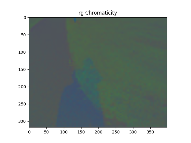
    # Visualize rg Chromaticity --> DEBUGGING
    rg_chrom = np.zeros_like(img)

    rg_chrom[:,:,0] = np.clip(np.uint8(rg_chrom_r*255), 0, 255)
    rg_chrom[:,:,1] = np.clip(np.uint8(rg_chrom_g*255), 0, 255)
    rg_chrom[:,:,2] = np.clip(np.uint8(rg_chrom_b*255), 0, 255)

    plt.imshow(rg_chrom)
    plt.title('rg Chromaticity')
    plt.show()

    #-----------------------
    ## 2. Take Logarithms ##
    #-----------------------

    l_rg = np.ma.log(n_r)
    l_bg = np.ma.log(n_b)

    log_r = np.ma.log(mean_r)
    log_g = np.ma.log(mean_g)
    log_b = np.ma.log(mean_b)

    ##  rho = np.zeros_like(img, dtype=np.float64)
    ##
    ##  rho[:,:,0] = log_r
    ##  rho[:,:,1] = log_g
    ##  rho[:,:,2] = log_b

    rho = cv2.merge((log_r, log_g, log_b))

    # Visualize Logarithms --> DEBUGGING
    plt.scatter(l_rg, l_bg, s = 2)
    plt.xlabel('Log(R/G)')
    plt.ylabel('Log(B/G)')
    plt.title('Log Chromaticities')
    plt.show()

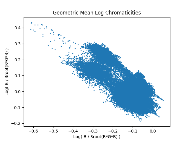
    plt.scatter(log_r, log_b, s = 2)
    plt.xlabel('Log( R / 3root(R*G*B) )')
    plt.ylabel('Log( B / 3root(R*G*B) )')
    plt.title('Geometric Mean Log Chromaticities')
    plt.show()

    #----------------------------
    ## 3. Rotate through Theta ##
    #----------------------------
    u = 1./np.sqrt(3)*np.array([[1,1,1]]).T
    I = np.eye(3)

    tol = 1e-15

    P_u_norm = I - u.dot(u.T)
    U_, s, V_ = np.linalg.svd(P_u_norm, full_matrices = False)

    s[ np.where( s <= tol ) ] = 0.

    U = np.dot(np.eye(3)*np.sqrt(s), V_)
    U = U[ ~np.all( U == 0, axis = 1) ].T

    # Columns are upside down and column 2 is negated...?
    U = U[::-1,:]
    U[:,1] *= -1.

    ##  TRUE ARRAY:
    ##
    ##  U = np.array([[ 0.70710678,  0.40824829],
    ##                [-0.70710678,  0.40824829],
    ##                [ 0.        , -0.81649658]])

    chi = rho.dot(U) 

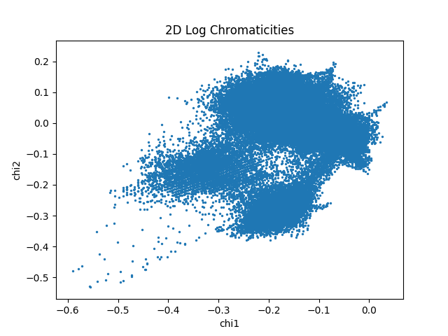
    # Visualize chi --> DEBUGGING
    plt.scatter(chi[:,:,0], chi[:,:,1], s = 2)
    plt.xlabel('chi1')
    plt.ylabel('chi2')
    plt.title('2D Log Chromaticities')
    plt.show()

    e = np.array([[np.cos(np.radians(np.linspace(1, 180, 180))), \
                   np.sin(np.radians(np.linspace(1, 180, 180)))]])

    gs = chi.dot(e)

    prob = np.array([np.histogram(gs[...,i], bins='scott', density=True)[0] 
                      for i in range(np.size(gs, axis=3))])

    eta = np.array([entropy(p, base=2) for p in prob])

    plt.plot(eta)
    plt.xlabel('Angle (deg)')
    plt.ylabel('Entropy, eta')
    plt.title('Entropy Minimization')
    plt.show()

    theta_min = np.radians(np.argmin(eta))

    print('Min Angle: ', np.degrees(theta_min))

    e = np.array([[-1.*np.sin(theta_min)],
                  [np.cos(theta_min)]])

    gs_approx = chi.dot(e)

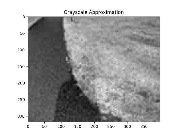
    # Visualize Grayscale Approximation --> DEBUGGING
    plt.imshow(gs_approx.squeeze(), cmap='gray')
    plt.title('Grayscale Approximation')
    plt.show()

    P_theta = np.ma.divide( np.dot(e, e.T), np.linalg.norm(e) )

    chi_theta = chi.dot(P_theta)
    rho_estim = chi_theta.dot(U.T)
    mean_estim = np.ma.exp(rho_estim)

    estim = np.zeros_like(mean_estim, dtype=np.float64)

    estim[:,:,0] = np.divide(mean_estim[:,:,0], np.sum(mean_estim, axis=2))
    estim[:,:,1] = np.divide(mean_estim[:,:,1], np.sum(mean_estim, axis=2))
    estim[:,:,2] = np.divide(mean_estim[:,:,2], np.sum(mean_estim, axis=2))

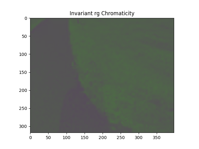
    plt.imshow(estim)
    plt.title('Invariant rg Chromaticity')
    plt.show()

Salida: