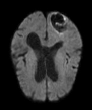
аюсь сделать автоматическую сегментацию изображения различных областей двухмерного изображения MR на основе значений интенсивности пикселей. Первым шагом является реализация модели гауссовой смеси на гистограмме изображения.

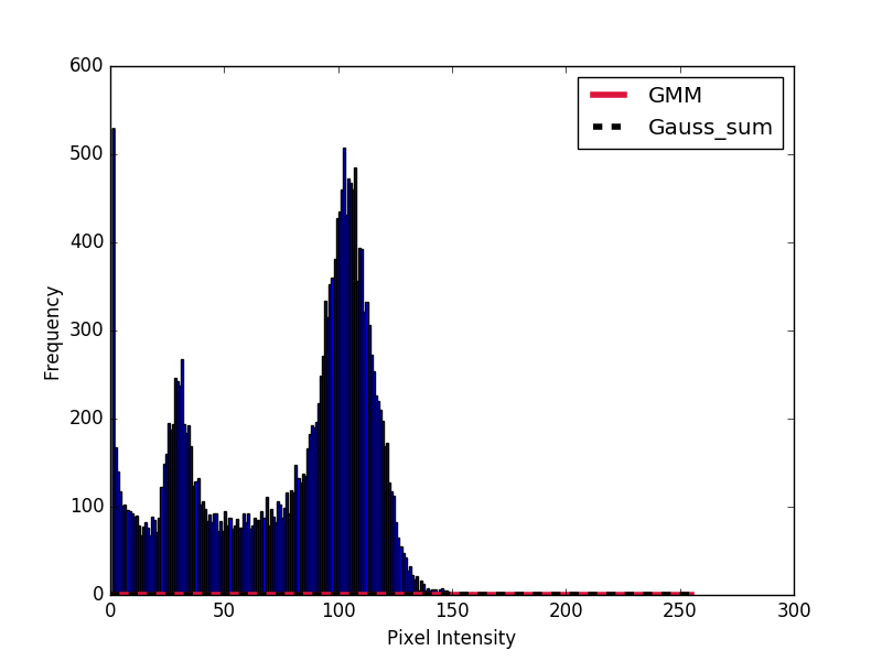
Мне нужно построить результирующий гауссиан, полученный изscore_samples метод на гистограмму. Я попытался, следуя коду в ответе (Понимание гауссовых моделей смесей).

Однако полученный гауссиан вообще не соответствует гистограмме. Как мне заставить гауссиан соответствовать гистограмме?

import numpy as np
import cv2
import matplotlib.pyplot as plt
from sklearn.mixture import GaussianMixture

# Read image
img = cv2.imread("test.jpg",0)

hist = cv2.calcHist([img],[0],None,[256],[0,256])
hist[0] = 0     # Removes background pixels

# Fit GMM
gmm = GaussianMixture(n_components = 3)
gmm = gmm.fit(hist)

# Evaluate GMM
gmm_x = np.linspace(0,255,256)
gmm_y = np.exp(gmm.score_samples(gmm_x.reshape(-1,1)))


# Plot histograms and gaussian curves
fig, ax = plt.subplots()
ax.hist(img.ravel(),255,[1,256])
ax.plot(gmm_x, gmm_y, color="crimson", lw=4, label="GMM")

ax.set_ylabel("Frequency")
ax.set_xlabel("Pixel Intensity")

plt.legend()

plt.show()

Я также попытался вручную построить гауссиан с суммами.

import numpy as np
import cv2
import matplotlib.pyplot as plt
from sklearn.mixture import GaussianMixture

def gauss_function(x, amp, x0, sigma):
    return amp * np.exp(-(x - x0) ** 2. / (2. * sigma ** 2.))

# Read image
img = cv2.imread("test.jpg",0)

hist = cv2.calcHist([img],[0],None,[256],[0,256])
hist[0] = 0     # Removes background pixels

# Fit GMM
gmm = GaussianMixture(n_components = 3)
gmm = gmm.fit(hist)

# Evaluate GMM
gmm_x = np.linspace(0,255,256)
gmm_y = np.exp(gmm.score_samples(gmm_x.reshape(-1,1)))

# Construct function manually as sum of gaussians
gmm_y_sum = np.full_like(gmm_x, fill_value=0, dtype=np.float32)
for m, c, w in zip(gmm.means_.ravel(), gmm.covariances_.ravel(), gmm.weights_.ravel()):
    gauss = gauss_function(x=gmm_x, amp=1, x0=m, sigma=np.sqrt(c))
    gmm_y_sum += gauss / np.trapz(gauss, gmm_x) * w

# Plot histograms and gaussian curves
fig, ax = plt.subplots()
ax.hist(img.ravel(),255,[1,256])
ax.plot(gmm_x, gmm_y, color="crimson", lw=4, label="GMM")
ax.plot(gmm_x, gmm_y_sum, color="black", lw=4, label="Gauss_sum", linestyle="dashed")

ax.set_ylabel("Frequency")
ax.set_xlabel("Pixel Intensity")

plt.legend()

plt.show()

С участиемax.hist(img.ravel(),255,[1,256], normed=True)