Масштабирование и подгонка к логнормальному распределению с использованием логарифмической оси в Python
У меня есть лог-нормально распределенный набор образцов. Я могу визуализировать образцы, используя гистограмму с линейной или логарифмической осью X. Я могу выполнить подгонку к гистограмме, чтобы получить PDF, а затем масштабировать ее до гистограммы на графике с линейной осью X, см. Такжеэтот ранее опубликованный вопрос.
Я, однако, не могу правильно построить PDF в график с логарифмической осью X.
К сожалению, это не только проблема с масштабированием области PDF к гистограмме, но и PDF также смещен влево, как вы можете видеть из следующего графика.
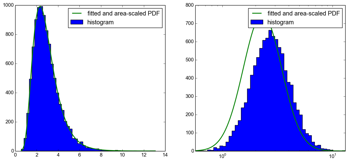
Мой вопрос сейчас, что я делаю не так здесь? Используя CDF для построения ожидаемой гистограммы,как предложено в этом ответе, работает. Я просто хотел бы знать, что я делаю неправильно в этом коде, так как в моем понимании он тоже должен работать.
Это код Python (извините, он довольно длинный, но я хотел опубликовать «полную автономную версию»):
import numpy as np
import matplotlib.pyplot as plt
import scipy.stats

# generate log-normal distributed set of samples
np.random.seed(42)
samples   = np.random.lognormal( mean=1, sigma=.4, size=10000 )

# make a fit to the samples
shape, loc, scale = scipy.stats.lognorm.fit( samples, floc=0 )
x_fit       = np.linspace( samples.min(), samples.max(), 100 )
samples_fit = scipy.stats.lognorm.pdf( x_fit, shape, loc=loc, scale=scale )

# plot a histrogram with linear x-axis
plt.subplot( 1, 2, 1 )
N_bins = 50
counts, bin_edges, ignored = plt.hist( samples, N_bins, histtype='stepfilled', label='histogram' )
# calculate area of histogram (area under PDF should be 1)
area_hist = .0
for ii in range( counts.size):
    area_hist += (bin_edges[ii+1]-bin_edges[ii]) * counts[ii]
# oplot fit into histogram
plt.plot( x_fit, samples_fit*area_hist, label='fitted and area-scaled PDF', linewidth=2)
plt.legend()

# make a histrogram with a log10 x-axis
plt.subplot( 1, 2, 2 )
# equally sized bins (in log10-scale)
bins_log10 = np.logspace( np.log10( samples.min()  ), np.log10( samples.max() ), N_bins )
counts, bin_edges, ignored = plt.hist( samples, bins_log10, histtype='stepfilled', label='histogram' )
# calculate area of histogram
area_hist_log = .0
for ii in range( counts.size):
    area_hist_log += (bin_edges[ii+1]-bin_edges[ii]) * counts[ii]
# get pdf-values for log10 - spaced intervals
x_fit_log       = np.logspace( np.log10( samples.min()), np.log10( samples.max()), 100 )
samples_fit_log = scipy.stats.lognorm.pdf( x_fit_log, shape, loc=loc, scale=scale )
# oplot fit into histogram
plt.plot( x_fit_log, samples_fit_log*area_hist_log, label='fitted and area-scaled PDF', linewidth=2 )

plt.xscale( 'log' )
plt.xlim( bin_edges.min(), bin_edges.max() )
plt.legend()
plt.show()
Обновление 1:
Я забыл упомянуть версии, которые я использую:
python      2.7.6
numpy       1.8.2
matplotlib  1.3.1
scipy       0.13.3
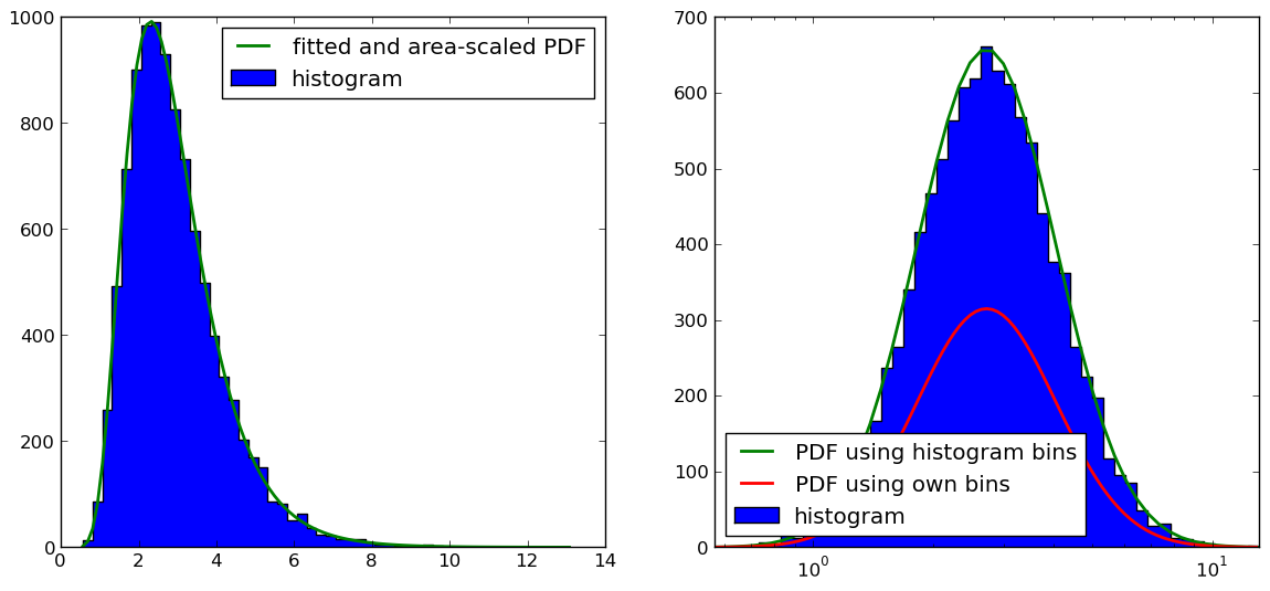
Обновление 2:
Как указали @Christoph и @zaxliu (спасибо обоим), проблема заключается в масштабировании PDF. Он работает, когда я использую те же ячейки, что и для гистограммы, как в решении @ zaxliu, но у меня все еще есть некоторые проблемы при использовании более высокого разрешения для PDF (как в моем примере выше). Это показано на следующем рисунке:
Код для рисунка справа (я пропустил материал для импорта и создания образца данных, который вы можете найти в приведенном выше примере):
# equally sized bins in log10-scale
bins_log10 = np.logspace( np.log10( samples.min()  ), np.log10( samples.max() ), N_bins )
counts, bin_edges, ignored = plt.hist( samples, bins_log10, histtype='stepfilled', label='histogram' )

# calculate length of each bin (required for scaling PDF to histogram)
bins_log_len = np.zeros( bins_log10.size )
for ii in range( counts.size):
    bins_log_len[ii] = bin_edges[ii+1]-bin_edges[ii]

# get pdf-values for same intervals as histogram
samples_fit_log = scipy.stats.lognorm.pdf( bins_log10, shape, loc=loc, scale=scale )

# oplot fitted and scaled PDF into histogram
plt.plot( bins_log10, np.multiply(samples_fit_log,bins_log_len)*sum(counts), label='PDF using histogram bins', linewidth=2 )

# make another pdf with a finer resolution
x_fit_log       = np.logspace( np.log10( samples.min()), np.log10( samples.max()), 100 )
samples_fit_log = scipy.stats.lognorm.pdf( x_fit_log, shape, loc=loc, scale=scale )
# calculate length of each bin (required for scaling PDF to histogram)
# in addition, estimate middle point for more accuracy (should in principle also be done for the other PDF)
bins_log_len       = np.diff( x_fit_log )
samples_log_center = np.zeros( x_fit_log.size-1 )
for ii in range( x_fit_log.size-1 ):
    samples_log_center[ii] = .5*(samples_fit_log[ii] + samples_fit_log[ii+1] )

# scale PDF to histogram
# NOTE: THIS IS NOT WORKING PROPERLY (SEE FIGURE)
pdf_scaled2hist = np.multiply(samples_log_center,bins_log_len)*sum(counts)

# oplot fit into histogram
plt.plot( .5*(x_fit_log[:-1]+x_fit_log[1:]), pdf_scaled2hist, label='PDF using own bins', linewidth=2 )

plt.xscale( 'log' )
plt.xlim( bin_edges.min(), bin_edges.max() )
plt.legend(loc=3)